- Records
- 592
- Columns
- 16
- Data through
- 2026
- Source updates
- annual
- Issue collected
- 2026-08-11
- Licence
- CC-BY-4.0
What you get
- 592-row CSV16 typed columns, ready for pandas, Excel or SQL
- PDF intelligence briefthe analytics read and methodology, written against this issue
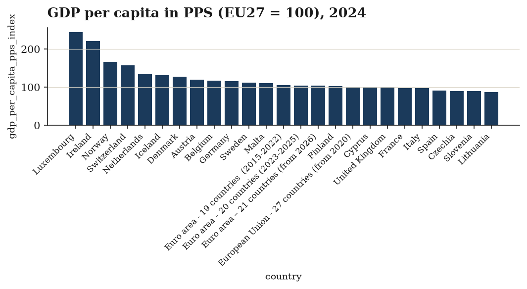
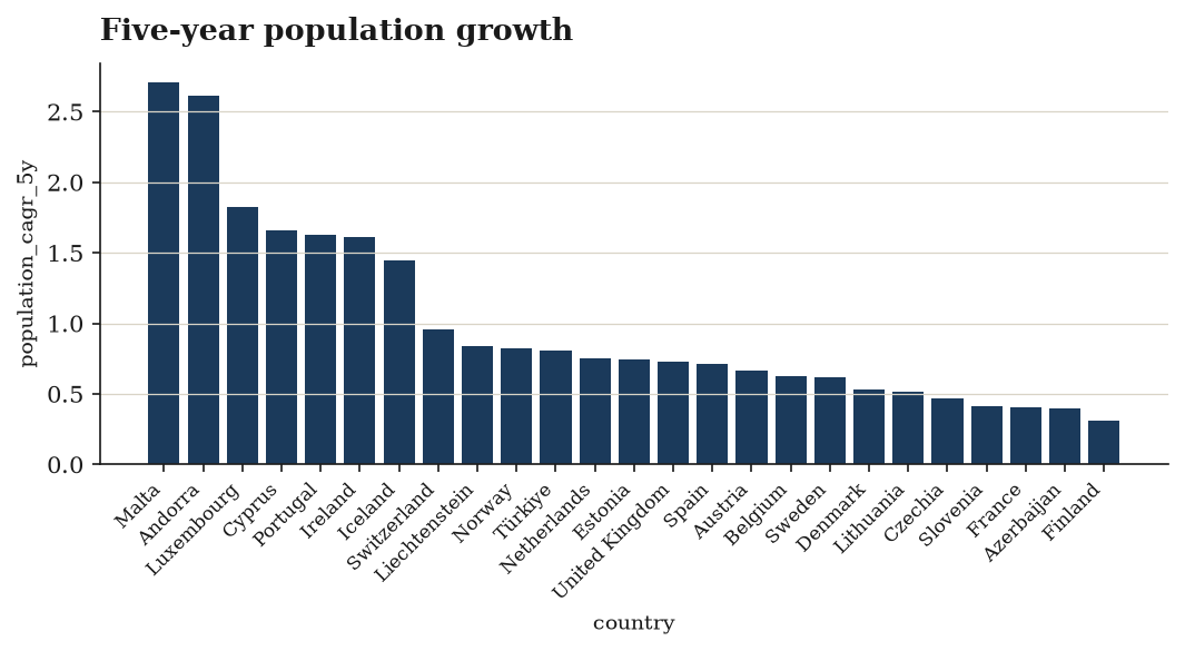
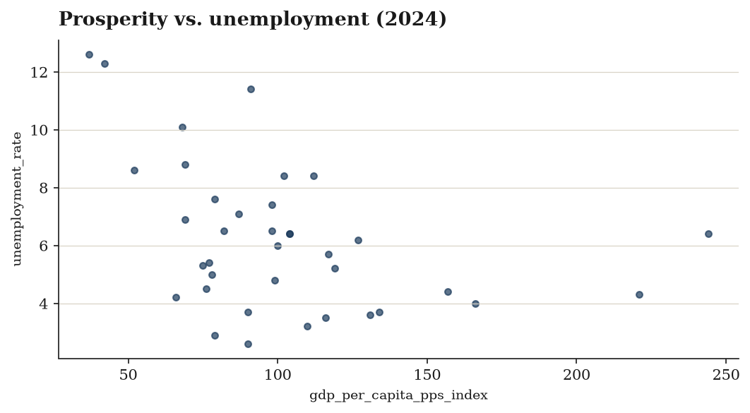
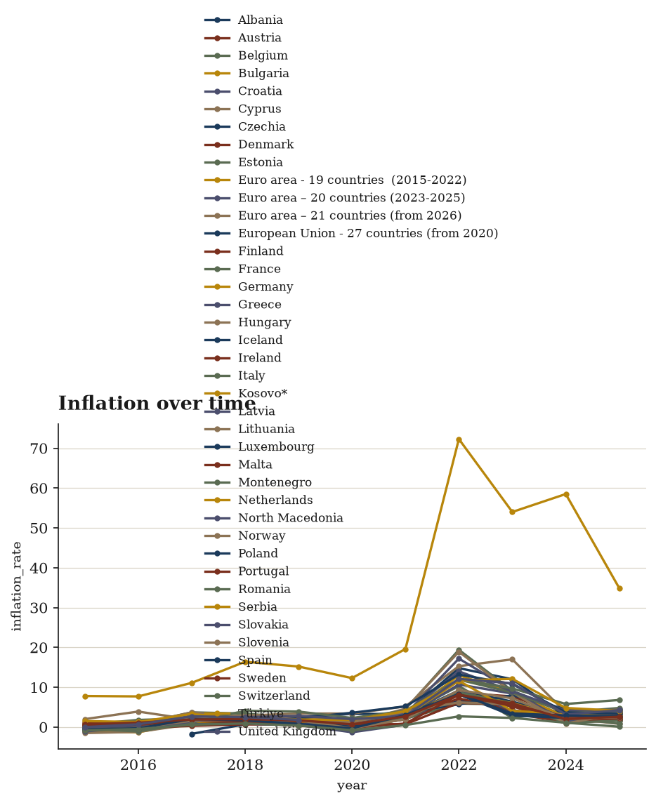
- 4 chartspublication-ready PNGs of the headline relationships
- analytics.md + statistics.mdthe same findings as text, for quoting and reuse
- Versioned archiveevery past issue stays downloadable, so you can build a time series
- API accesspull the data with a scoped key instead of clicking download
What the current issue shows
Extreme scale dispersion in population. Values run from 32,790 to 452 million, with a mean of 43.2m against a median of 6.45m and a standard deviation of 100.1m — a heavily right-skewed distribution consistent with the presence of aggregate entities alongside micro-states. population_share_pct mirrors this: median 0.31% but a maximum of 26.04%.
Wide prosperity gap.gdp_per_capita_pps_index spans 30 to 279 (mean 97.95, median 95, stdev 43.78) — a near ten-fold range between the poorest and richest observations, centred close to the index base of 100.
Inflation is the most volatile series. It ranges from −1.7% (deflation) to 72.3%, with a median of 2.1% but a mean of 3.53% and stdev 6.24 — a small number of hyperinflationary observations drag the mean well above the typical case. This feeds directly into the misery_index, whose maximum of 82.8 dwarfs its median of 9.1.
Labour markets diverge sharply. Unemployment runs 2% to 26.1% (median 6.5%, mean 7.55%).
Demographic decline is common but not dominant.population_cagr_5y averages just +0.24% (median +0.30%) with a floor of −5.46% and ceiling of +3.25%; 116 of 592 rows (19.6%) are flagged is_shrinking. 154 rows (26.0%) are flagged is_under_pressure.
Weak average growth.gdp_growth_cagr_5y averages 0.74% (median 0.43%), from −2.12% to +7.47%.
Charts included
Data preview
| geo_code | country | year | population | gdp_per_capita_pps_index | inflation_rate | unemployment_rate |
|---|---|---|---|---|---|---|
| AD | Andorra | 2016 | 71732.0 | |||
| AD | Andorra | 2018 | 74794.0 | |||
| AD | Andorra | 2019 | 76177.0 | |||
| AD | Andorra | 2020 | 77543.0 | |||
| AD | Andorra | 2022 | 79535.0 | |||
| AD | Andorra | 2023 | 81588.0 | |||
| AD | Andorra | 2024 | 85101.0 | |||
| AD | Andorra | 2026 | 89058.0 |
First 8 of 592 rows and 9 further columns. The download carries every row and column.
Every column, defined
geo_codecountryyearpopulation(persons) — population on 1 Januarygdp_per_capita_pps_index— GDP per capita in PPS, EU27 = 100inflation_rate(%) — HICP annual average rate of changeunemployment_rate(%) — unemployment, 15-74, both sexes, % of active populationpopulation_cagr_5y(%) — 5-year compound population growthpopulation_share_pct(%) — country share of the cohort population that yeargdp_growth_cagr_5y(%) — 5-year compound growth of the GDP-per-capita indexmisery_index— inflation + unemployment — the classic household-pressure gaugeprosperity_zscore— standardised GDP per capita across the cohortstability_score— 0-100 composite: high output, low inflation, low unemploymenteconomy_class— leading | above-average | catching-up | laggingis_shrinking— population contracting over the last five yearsis_under_pressure— misery index above 10
Inside the PDF brief
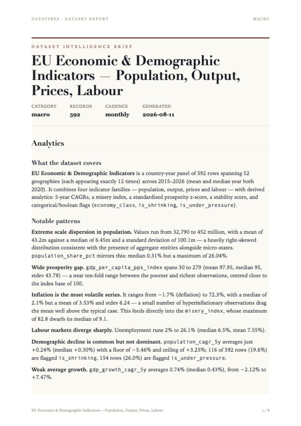
Every issue ships with a written brief: what the data covers, the patterns worth acting on, and the statistical work behind each derived column — with the limitations stated plainly rather than buried.
The page shown here is the first of the full report included in your download. Tap it to read at full size.
Method and limitations
1. Dataset Scope
The eu-economic-demographic dataset (category: macro) contains 592 rows describing 52 geographies (geo_code / country) over the years 2015–2026 (mean = 2020, median = 2020, stdev = 3.443). Each geography appears exactly 12 times, indicating a balanced country × year panel (52 × 12 = 624 potential cells versus 592 observed rows, so some cells are absent).
Base (input) measures:
| Measure | Unit | Coverage | Range |
|---|---|---|---|
population | persons | 592/592 | 3.279e+04 – 4.52e+08 |
gdp_per_capita_pps_index | index | 449/592 | 30 – 279 |
inflation_rate | % | 436/592 | −1.7 – 72.3 |
unemployment_rate | % | 406/592 | 2 – 26.1 |
2. Preparation Steps
- Normalize — column/value standardisation applied prior to any statistical derivation.
- Join on the composite key
['geo_code', 'year'], combining the population, output, price and labour sources into a single panel row per country-year. - Filter to rows where
populationis not null. This makespopulationand its derived share fully populated (592/592) and defines the analytical universe; all other indicators retain missingness. - Sort by
['geo_code', 'year']— a prerequisite for the ordered, within-country growth calculations that follow.
3. Derived Statistics
3.1 Compound annual growth rates (within-country)
population_cagr_5y=cagr(population, years=5), partitioned bygeo_code.gdp_growth_cagr_5y=cagr(gdp_per_capita_pps_index, years=5), partitioned bygeo_code.
Both are annualised 5-year compound growth rates computed inside each country's time-ordered series, so no cross-country contamination occurs. The 5-year lookback consumes the earliest years of each series, which is reflected in reduced coverage: population CAGR is present for 332/592 rows (mean 0.241 %, median 0.296 %, range −5.461 % to 3.248 %) and GDP-per-capita CAGR for only 244/592 rows (mean 0.739 %, median 0.432 %, range −2.117 % to 7.466 %) — the latter further limited by the 449-row base coverage of the index.
3.2 Cross-sectional composition
population_share_pct=share_of_total(population), partitioned byyear.
Each country's population is expressed as a percentage of the total population of all countries present in that same year, so shares are internally comparable within a year. Values span 0.0015 % to 26.04 %, with mean 2.027 % and median 0.306 % — a strongly right-skewed distribution consistent with the population column itself (mean 4.319e+07 vs. median 6.447e+06).
3.3 Standardisation
prosperity_zscore=zscore(gdp_per_capita_pps_index), computed globally (nobyclause).
The resulting column has mean ≈ 0 (1.295e−16, i.e. floating-point zero) and stdev = 1.000, confirming a single pooled standardisation over all 449 non-null index observations. Its range (−1.552 to 4.135) is markedly asymmetric to the upside, and the negative median (−0.0674) indicates a right-skewed prosperity distribution: a few very high-index geographies (max index 279) pull the mean above the typical country.
3.4 Additive composite: misery index
misery_index=add(inflation_rate, unemployment_rate).
A simple unweighted sum of two percentage-point rates, defined only where both inputs exist — hence 399/592 non-null rows (fewer than either parent column: 436 and 406). Mean 11.06, median 9.1, maximum 82.8; the high maximum is traceable to the inflation maximum of 72.3 %.
3.5 Weighted composite: stability score
stability_score= weighted score on a 0–100 scale with weightsgdp_per_capita_pps_index= 0.6,unemployment_rate= 0.2,inflation_rate= 0.2.
Output coverage is 456/592, mean 22.07, median 21.86, stdev 10.12, range 0 – 64.39. The near-equality of mean and median suggests an approximately symmetric distribution after scaling. The 0.6 weight makes relative output per capita the dominant contributor, with labour and price conditions sharing the remaining 0.4 equally.
4. Classification and Flags
4.1 Banding of output per capita
economy_class is assigned from gdp_per_capita_pps_index using ordered, upper-open bins:
| Label | Rule | Rows |
|---|---|---|
| leading | index ≥ 125 | 83 |
| above-average | 100 ≤ index < 125 | 117 |
| catching-up | 75 ≤ index < 100 | 117 |
| lagging | index < 75 | 132 |
| unknown | default (index missing) | 143 |
The 143 unknown rows equal exactly the 592 − 449 rows with a missing index, so the default branch is functioning purely as a missing-data sentinel. unknown is the modal category, and lagging is the largest substantive class.
4.2 Boolean flags
is_shrinking=population_cagr_5y < 0→ 116 True, 476 False.is_under_pressure=misery_index > 10→ 154 True, 438 False.
Both are strict, single-threshold rules on derived columns.
4.3 Validation
A terminal validate step closes the pipeline, consistent with the observed internal coherence (z-score mean ≈ 0 and stdev = 1; unknown count matching index missingness; full coverage of population and population_share_pct).
5. Limitations
Missing-data propagation. Coverage degrades sharply down the derivation chain: 449 rows for the index, 436 for inflation, 406 for unemployment, 399 for the misery index, 332 for population CAGR, and only 244 for GDP CAGR. Any statistic built on the scarcer columns describes a shrinking, non-random subset of the panel — not the 592-row universe.
Only population was required to be non-null. The filter guarantees demographic completeness alone. Consequently the population-based columns are fully populated while every economic column carries gaps, creating asymmetric comparability between demographic and economic conclusions.
False negatives in boolean flags.is_shrinking and is_under_pressure are stored as booleans with only True/False values. Rows with a missing population_cagr_5y (260 rows) or missing misery_index (193 rows) cannot satisfy the conditions and therefore fall into False. The 476 "not shrinking" and 438 "not under pressure" counts thus conflate genuine negatives with unknowns and should not be read as measured absences.
unknown is not an economic category. All 143 unknown rows arise from a missing index, so economy_class mixes a measurement-status label with four substantive bands. Distributions over economy_class are only interpretable after excluding unknown.
Truncated growth windows. The 5-year CAGRs cannot be computed for the earliest years of each country series, so growth-based statistics are systematically biased toward later years within the 2015–2026 span. With years extending to 2026 while the panel is dated as-is, later observations may rest on projections rather than outturns; the dataset provides no field distinguishing observed from forecast values.
Two-point nature of CAGR. A compound annual growth rate depends only on the endpoints of its window and ignores the intervening path. Volatility, reversals and one-off level breaks are invisible; the extreme population CAGR of −5.461 % cannot be distinguished from a definitional or boundary change on the available fields.
Composite index construction. The misery_index sums two percentage rates with implicit equal weight and no normalisation, so it is dominated by whichever component has the larger spread — here inflation, whose range (−1.7 to 72.3) far exceeds unemployment's (2 to 26.1). Its 82.8 maximum reflects a single inflation extreme rather than broad-based distress. The stability_score weights (0.6 / 0.2 / 0.2) are analyst-chosen rather than empirically estimated, and the pipeline record does not state the direction of each component's contribution or the pre-scaling transformation, so the 0–100 values are ordinal-comparable at best.
Pooled standardisation.prosperity_zscore is computed over all country-years at once, without a by partition. It therefore mixes cross-sectional and temporal variation: a score reflects position relative to the whole 2015–2026 pool, not relative to peers in the same year, and it is not a like-for-like measure of within-year relative prosperity. Its skew (median −0.0674, max +4.135) also means z-scores are not symmetric around the typical country.
Shares are relative to observed rows only.population_share_pct divides by the total of countries present in each year. If country coverage differs across years, the denominator shifts and shares are not strictly comparable over time. Shares also sum to 100 % per year by construction, so they measure composition, not absolute demographic change.
Skew and outlier sensitivity. Population spans four orders of magnitude (3.279e+04 to 4.52e+08) with mean far above median, so unweighted cross-country means of any indicator treat micro-geographies and the largest entity equally. No population weighting is applied anywhere in the pipeline.
Unit heterogeneity in geography. With 52 distinct geo_code values and a maximum population of 4.52e+08 (26.04 % of a year's total), the panel appears to mix individual countries with at least one aggregate entity. Aggregates and their members counted together would double-count in any total, mean or share computed across all rows.
Undocumented steps. The normalize, join and validate operations are recorded without parameters or rule definitions (beyond the join keys). Join behaviour for unmatched keys, and the validation criteria and their pass/fail outcome, cannot be verified from the information provided.
No inference performed. The pipeline produces descriptive derivations, composites, bands and flags only. There are no confidence intervals, significance tests or controls, and no correlation or causal estimation. Nothing here supports statements about what drives prosperity, growth or stability.
Provenance
Source: Eurostat: tps00001 (population), tec00114 (GDP per capita PPS), tec00118 (HICP), une_rt_a (unemployment)
Licence: Eurostat open data — free reuse with attribution (CC-BY-4.0 equivalent)
Collected and derived with datavibes, a deterministic pipeline: the same config and timestamp always reproduce the same file.