- Records
- 1,268
- Columns
- 14
- Data through
- 2026-08-11
- Source updates
- daily
- Issue collected
- 2026-08-11
- Licence
- CC-BY-4.0
What you get
- 1,268-row CSV14 typed columns, ready for pandas, Excel or SQL
- PDF intelligence briefthe analytics read and methodology, written against this issue
- 4 chartspublication-ready PNGs of the headline relationships
- analytics.md + statistics.mdthe same findings as text, for quoting and reuse
- Versioned archiveevery past issue stays downloadable, so you can build a time series
- API accesspull the data with a scoped key instead of clicking download
What the current issue shows
- Wide price dispersion.
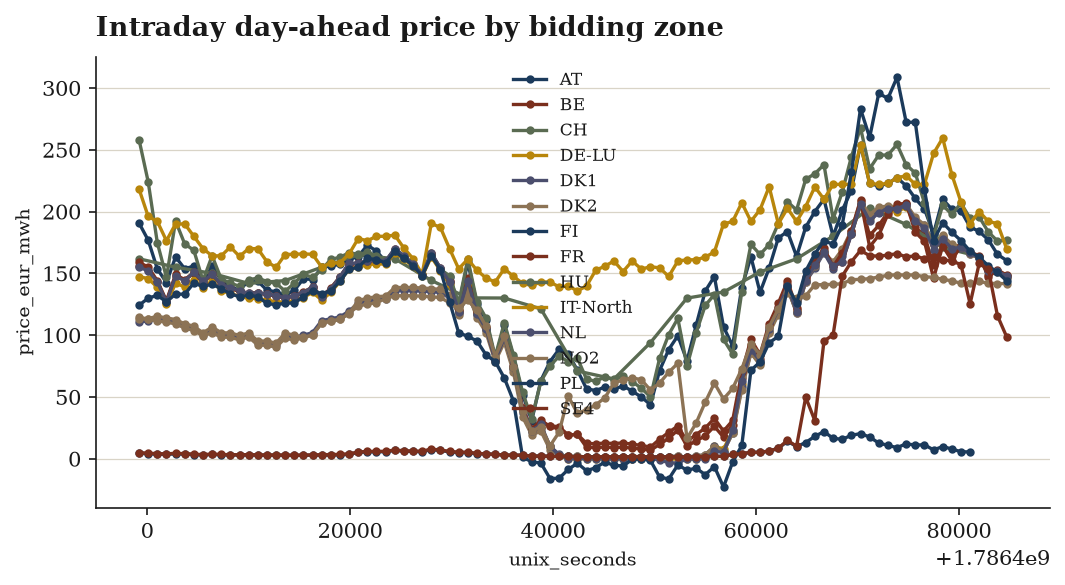
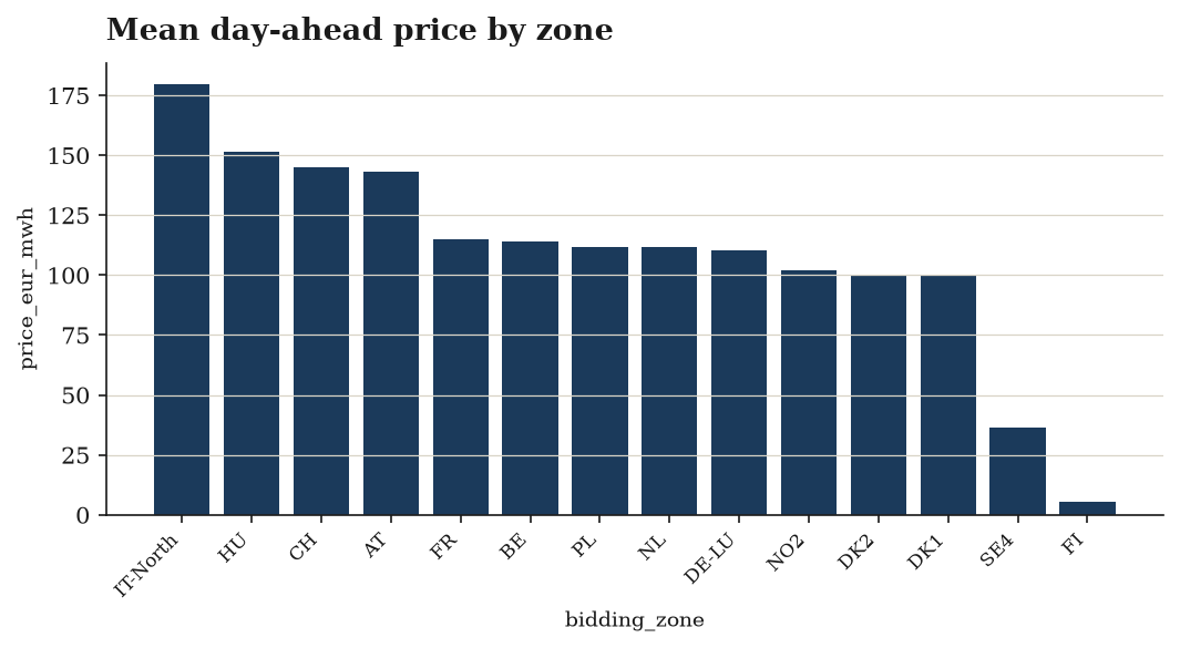
price_eur_mwhranges from −22.87 to 308.60 EUR/MWh with stdev 71.32. The mean (107.3) sits well below the median (130.5), indicating a left-skewed distribution dragged down by a cluster of cheap and negative intervals. - Band distribution is top-heavy.
expensivedominates at 676 rows (53%), followed bycheap(295),normal(235),negative(49) andextreme(13). Only ~19% of intervals are "normal" — this is a volatile day by construction. - Negative pricing is material. 42 rows are flagged
is_negative_price(3.3%). Note the discrepancy with the 49 rows in thenegativeprice band — worth reconciling before use, as the two fields apply different thresholds or logic. - Volatility clustering.
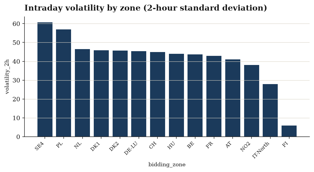
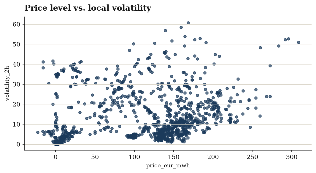
is_high_volatilityis True for 212 rows (16.7%), while spikes are rarer at 29 rows (2.3%).volatility_6hreaches 111.6 EUR/MWh against a median of 26.04, so extreme regimes are concentrated rather than diffuse. - Expected rolling-window gaps.
volatility_2hhas 98 nulls andvolatility_6hhas 322 nulls (25%) — approximately 23 warm-up rows per zone across 14 zones.price_change_pcthas 21 nulls (first observation per zone). Oneprice_change_pctoutlier hits +47 (4700%), almost certainly a rebound off a near-zero or negative price; treat percentage changes with care in negative-price regimes. - Normalisation is clean:
price_vs_day_meanandprice_zscoreboth centre on zero, confirming per-day standardisation.
Charts included
Data preview
| bidding_zone | unix_seconds | price_eur_mwh | price_change_pct | volatility_2h | volatility_6h | price_vs_day_mean |
|---|---|---|---|---|---|---|
| AT | 1786399200 | 190.73 | 47.44291666666666 | |||
| AT | 1786400100 | 176.89 | -0.07256330939023753 | 33.60291666666666 | ||
| AT | 1786401000 | 153.64 | -0.1314376165978857 | 10.352916666666658 | ||
| AT | 1786401900 | 142.55 | -0.07218172350950258 | -0.7370833333333167 | ||
| AT | 1786402800 | 163.27 | 0.1453525078919677 | 19.982916666666682 | ||
| AT | 1786403700 | 153.72 | -0.058492068353034915 | 10.43291666666667 | ||
| AT | 1786404600 | 155.91 | 0.01424668227946915 | 12.622916666666669 | ||
| AT | 1786405500 | 142.42 | -0.08652427682637424 | 16.692078050466247 | -0.8670833333333405 |
First 8 of 1,268 rows and 7 further columns. The download carries every row and column.
Every column, defined
bidding_zone— ENTSO-E bidding-zone codeunix_seconds— start of the quarter-hourly interval, UTC epoch secondsprice_eur_mwh(EUR/MWh) — day-ahead spot price for the intervalprice_change_pct— fractional change vs. the previous intervalvolatility_2h(EUR/MWh) — trailing 8-interval (2-hour) standard deviationvolatility_6h(EUR/MWh) — trailing 24-interval (6-hour) standard deviationprice_vs_day_mean(EUR/MWh) — deviation from the zone's mean price for the dayprice_zscore— standardised price within the zone's dayrolling_avg_2h(EUR/MWh)intraday_position— 0-1 where the interval sits between the zone's daily low and highprice_band— negative | cheap | normal | expensive | extremeis_negative_price— oversupply — generators pay to deliveris_price_spike— more than two standard deviations above the zone's daily meanis_high_volatility— 2-hour volatility above 25 EUR/MWh
Inside the PDF brief
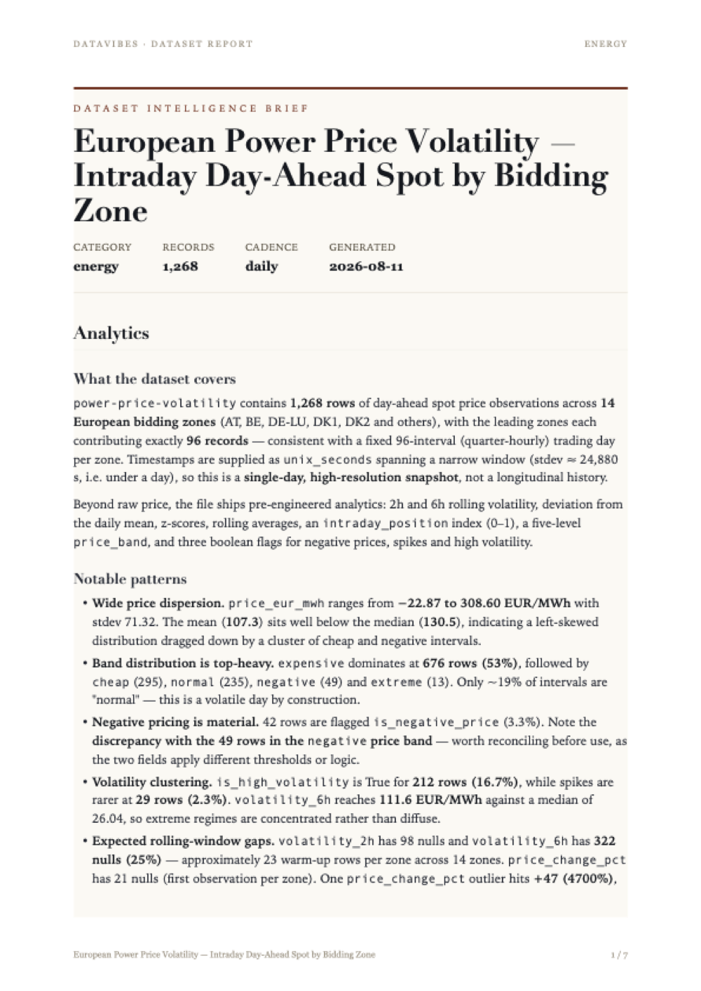
Every issue ships with a written brief: what the data covers, the patterns worth acting on, and the statistical work behind each derived column — with the limitations stated plainly rather than buried.
The page shown here is the first of the full report included in your download. Tap it to read at full size.
Method and limitations
Dataset Context
The dataset (power-price-volatility, energy category) holds 1,268 records of day-ahead spot prices in EUR/MWh across 14 European bidding zones. Zone coverage is balanced at the top of the frequency table — AT, BE, DE-LU, DK1 and DK2 each contribute 96 rows — and the unix_seconds timestamp column spans a narrow window (stdev ≈ 2.49e+04 seconds, roughly a single day of quarter-hourly or hourly slots). Raw prices range from -22.87 to 308.6 EUR/MWh, with mean 107.3 and median 130.5, indicating a left-skewed distribution where a tail of low and negative prices pulls the mean below the median.
Preparation Prior to Derivation
- Normalize — schema/type harmonisation applied to all columns.
- Dedupe on the composite key
(bidding_zone, unix_seconds), enforcing one price observation per zone per timestamp. This is the key that makes all subsequent per-zone series well-defined. - Filter to rows where
price_eur_mwhis non-null. Consistent with this,price_eur_mwhis 1268/1268 non-null in the final profile. - Sort by
bidding_zone, thenunix_seconds— a prerequisite for any lag- or window-based statistic, since ordering determines what "previous" and "trailing window" mean.
All derivations below are computed grouped by bidding_zone (by: ['bidding_zone']), so no statistic mixes observations across market areas.
Derived Statistics
Period-over-period return
price_change_pct = pct_change(price_eur_mwh) — the fractional change against the preceding timestamp within the same zone. The first observation of each zone has no predecessor, which accounts for the 21 nulls (1247/1268 non-null). Distribution: mean 0.128, median -0.002851, min -4.996, max 47.0, stdev 1.807. The near-zero median against a positive mean and a maximum of 47 shows the metric is dominated by a few extreme ratios — a structural consequence of dividing by prices that approach zero.
Trailing volatility at two horizons
volatility_2h = volatility(price_eur_mwh, window=8)— rolling dispersion over 8 preceding observations. 1170/1268 non-null (98 nulls from window warm-up across the 14 zones). Mean 13.27, median 9.289, range 0.07251–60.64 EUR/MWh.volatility_6h = volatility(price_eur_mwh, window=24)— the same statistic over 24 observations. 946/1268 non-null (322 nulls, the larger warm-up cost of the wider window). Mean 31.63, median 26.04, range 0.4006–111.6 EUR/MWh.
Both are right-skewed (mean above median). The longer window reports systematically larger dispersion, as expected when a wider span admits more of the intraday price shape.
Rolling level
rolling_avg_2h = rolling_avg(price_eur_mwh, window=8) — trailing 8-observation mean, sharing the volatility_2h window and therefore its 1170/1268 coverage. Mean 104.7, median 128, range -11.89 to 276.9 EUR/MWh. Smoothing compresses the range relative to raw prices (which reach 308.6 and -22.87) and the mean sits close to the raw mean of 107.3.
Centring and standardisation
price_vs_day_mean = anomaly(price_eur_mwh)— deviation of each price from its zone mean. Fully populated (1268/1268). Mean is -1.22e-15, i.e. zero to floating-point precision, confirming the per-zone centring. Range -134.6 to 196.9 EUR/MWh, stdev 57.12.price_zscore = zscore(price_eur_mwh)— the same deviation scaled by the zone standard deviation. Mean -3.856e-17 and stdev 0.9949, both consistent with a correctly standardised variable. Range -2.435 to 3.425; median 0.1664 again reflects the left skew.
Positional index
intraday_position = minmax_normalize(price_eur_mwh) — each price rescaled to [0, 1] against its own zone's observed min and max. Observed bounds are exactly 0 and 1 (each zone contributes its own extremes), mean 0.4615, median 0.5134, stdev 0.312.
Classification and Flags
price_band bins raw price into five ordered, mutually exclusive labels via upper-bound cuts (default unknown, unused in the result):
| Band | Rule | Count |
|---|---|---|
| negative | price ≤ 0 | 49 |
| cheap | 0 < price ≤ 40 | 295 |
| normal | 40 < price ≤ 120 | 235 |
| expensive | 120 < price ≤ 250 | 676 |
| extreme | price > 250 | 13 |
expensive is the modal band at 676 of 1268 rows (~53%), which is coherent with a median price of 130.5 falling inside that interval.
Three booleans encode threshold events:
is_negative_price—price_eur_mwh < 0: 42 True, 1226 False.is_price_spike—price_zscore > 2: 29 True, 1239 False. Defined on the standardised series, so it is a relative spike within a zone, not an absolute price level.is_high_volatility—volatility_2h > 25EUR/MWh: 212 True, 1056 False.
A validate step closes the pipeline.
Limitations
- Warm-up nulls are unevenly distributed across metrics.
volatility_6his missing for 322 rows (25% of the dataset) andvolatility_2h/rolling_avg_2hfor 98. Any comparison of the two volatility horizons, or of volatility against price, is drawn from different row subsets unless explicitly restricted to complete cases. is_high_volatilityinherits those gaps. Rows wherevolatility_2his null cannot satisfy> 25, so they fall into the False bucket. The 1056 False count therefore conflates "measured as low volatility" with "not measurable".price_change_pctis unstable near zero prices. With prices reaching -22.87 and crossing zero, the denominator can be arbitrarily small; the maximum of 47 (a 4,700% move) and the mean/median divergence are artefacts of this rather than descriptions of typical behaviour. Sign flips across zero also make the percentage uninterpretable in direction.- Standardisation assumes a meaningful per-zone scale.
price_zscoreandintraday_positionare computed against each zone's own distribution over this single short window (~96 observations per zone). Thresholds likez > 2are relative to that small sample, so spike counts are not comparable to a longer historical baseline, andintraday_positionis anchored to extremes that are themselves sample-specific. - Short time span limits generalisation. The timestamp stdev of ~2.49e+04 seconds implies roughly one day of coverage. No seasonality, weekday effect, or multi-day mean reversion can be estimated from this data; "day mean" in
price_vs_day_meanis effectively the whole-sample zone mean. - Band cut-points are exogenous. The 0/40/120/250 EUR/MWh boundaries are fixed absolute levels, not data-driven quantiles. They are applied uniformly across all 14 zones despite differing price levels, which is why one band absorbs over half the rows and
extremeholds only 13 — small-cell counts unsuited to stratified inference. - Flag definitions overlap and are not independent.
is_negative_price(42) and thenegativeband (49) are built from the same underlying variable with different comparison operators (< 0versus≤ 0), and the seven-row difference reflects that boundary treatment rather than a data discrepancy. Similarlyis_price_spikeand theextremeband both mark high prices by different constructions and should not be treated as corroborating signals. - No causal or exogenous content. Nothing in the pipeline includes load, generation mix, interconnector flows or fuel prices, so the metrics describe price behaviour only and support no attribution of its drivers.
Provenance
Source: energy-charts.info day-ahead spot price API (Fraunhofer ISE)
Licence: CC-BY-4.0 (Fraunhofer ISE energy-charts; source data Bundesnetzagentur/SMARD, ENTSO-E)
Collected and derived with datavibes, a deterministic pipeline: the same config and timestamp always reproduce the same file.