- Records
- 208
- Columns
- 16
- Data through
- 2025
- Source updates
- annual
- Issue collected
- 2026-08-11
- Licence
- CC-BY-4.0
What you get
- 208-row CSV16 typed columns, ready for pandas, Excel or SQL
- PDF intelligence briefthe analytics read and methodology, written against this issue
- 4 chartspublication-ready PNGs of the headline relationships
- analytics.md + statistics.mdthe same findings as text, for quoting and reuse
- Versioned archiveevery past issue stays downloadable, so you can build a time series
- API accesspull the data with a scoped key instead of clicking download
What the current issue shows
- Extreme cost dispersion. ICT hourly cost ranges from €8.2 to €73.9 (mean 38.11, median 35.70, stdev 16.19) — roughly a 9x spread across the EU-scale sample. Wages follow the same shape (€7.1–€60.4, mean 30.44). The mean exceeding the median signals a right-skewed tail of high-cost markets, consistent with the z-score median of −0.149.
- ICT commands a premium everywhere.
ict_premium_pctnever falls below 110% (max 239.8, mean 149.1, median 136.6). No country-year in the sample pays ICT workers at or below the all-sector average — a clean, consistent finding for talent-cost modelling. - Wage share is stable, cost structure is not.
wage_cost_pctclusters tightly (mean 81.02, median 80.86, stdev 7.20) but spans 64.32%–96.2%, pointing to large differences in non-wage employer burdens. - Growth is volatile.
ict_cost_cagr_3yruns from −0.79% to 34.54% (mean 7.37, stdev 5.38) — at least one market with essentially flat ICT costs alongside extreme escalation elsewhere. - Purchasing power divergence. GDP per capita PPS index spans 44 to 262 (mean 103.5), while
cost_vs_purchasing_powerranges 0.131–0.604 — the affordability of local tech talent varies ~4.6x. - Value score spread is the headline.2.75 to 93.59 (mean 38.29, median 33.79) — a wide, decision-ready ranking signal.
- Tiering skews expensive: premium (81) and mid (80) dominate; only 6 rows are low-cost. 92 rows sit above the EU median cost vs 116 below.
Charts included
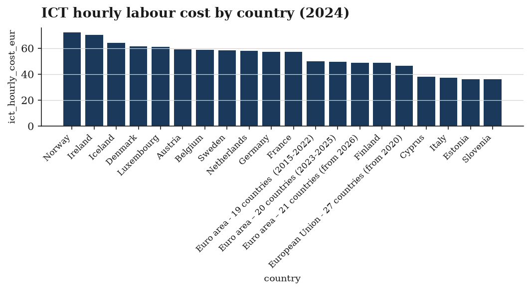
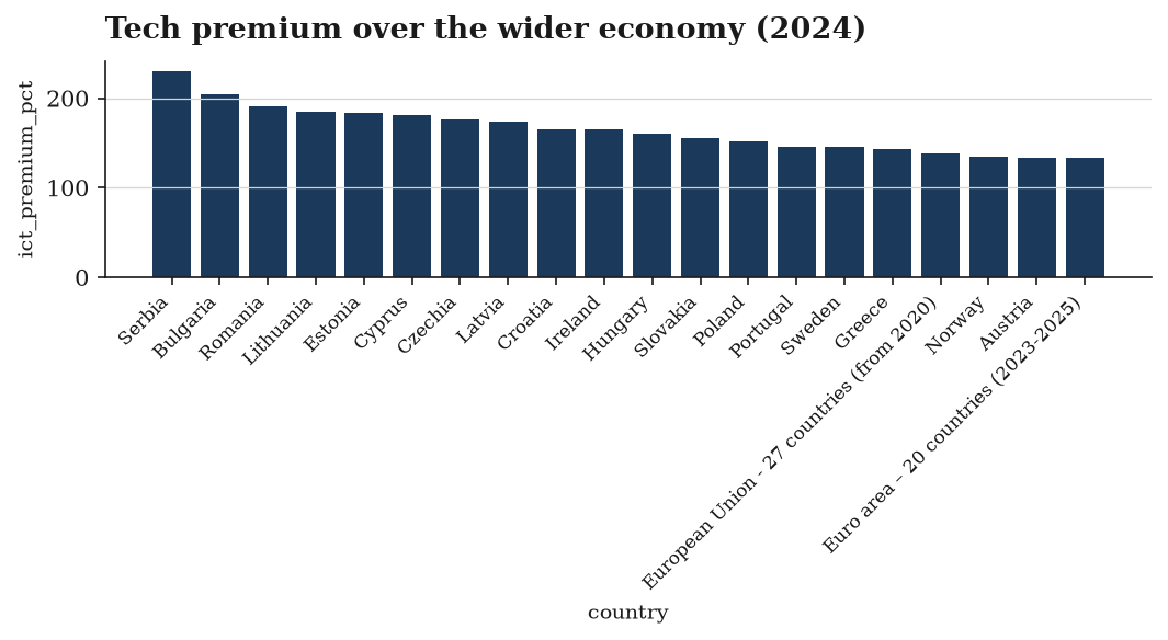
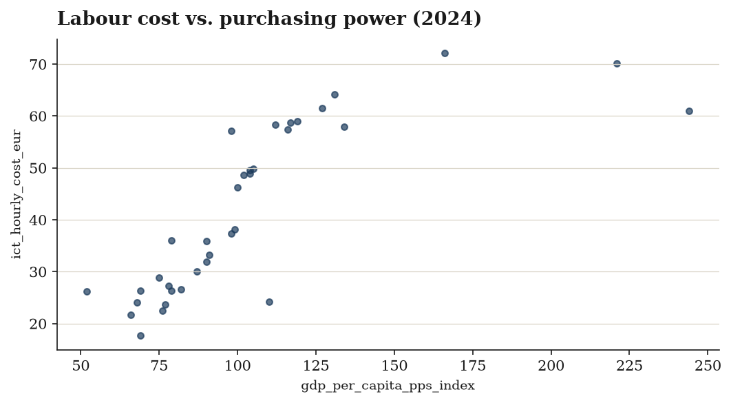
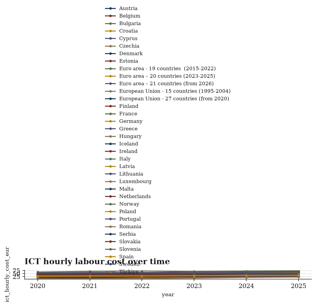
Data preview
| geo_code | country | year | ict_hourly_cost_eur | ict_hourly_wages_eur | all_sector_hourly_cost_eur | gdp_per_capita_pps_index |
|---|---|---|---|---|---|---|
| AT | Austria | 2020 | 49.2 | 36.8 | 36.4 | 123.0 |
| AT | Austria | 2021 | 47.5 | 35.0 | 36.7 | 121.0 |
| AT | Austria | 2022 | 51.0 | 37.7 | 38.5 | 123.0 |
| AT | Austria | 2023 | 53.9 | 39.9 | 41.3 | 121.0 |
| AT | Austria | 2024 | 59.0 | 43.9 | 44.3 | 119.0 |
| AT | Austria | 2025 | 61.6 | 45.5 | 46.3 | 118.0 |
| BE | Belgium | 2020 | 49.7 | 36.3 | 40.5 | 118.0 |
| BE | Belgium | 2021 | 50.2 | 36.7 | 41.0 | 116.0 |
First 8 of 208 rows and 9 further columns. The download carries every row and column.
Every column, defined
geo_codecountryyearict_hourly_cost_eur(EUR/hour) — total hourly labour cost, NACE J (information & communication)ict_hourly_wages_eur(EUR/hour) — wages and salaries component only, NACE Jall_sector_hourly_cost_eur(EUR/hour) — total hourly labour cost, business economy excluding public administration (NACE B-S_X_O)gdp_per_capita_pps_index— GDP per capita in PPS, EU27=100 — the purchasing-power anchorict_premium_pct(%) — ICT cost as a percent of the all-sector cost — 130 = a 30% tech premiumwage_cost_pct(%) — wages and salaries as a share of total ICT labour cost — the remainder is employer social contributionsict_cost_cagr_3y(%) — 3-year compound growth of ICT hourly labour costcost_vs_purchasing_power— ICT hourly cost ÷ GDP-per-capita index — high = expensive relative to local economic strengthcost_zscore— standardised ICT hourly cost across the cohortcost_index— 0-1 min-max ICT hourly cost within the cohortvalue_score— 0-100 hiring-value composite: cheap ICT labour in a strong economy scores highcost_tier— premium | high | mid | low-costis_above_eu_median_cost
Inside the PDF brief
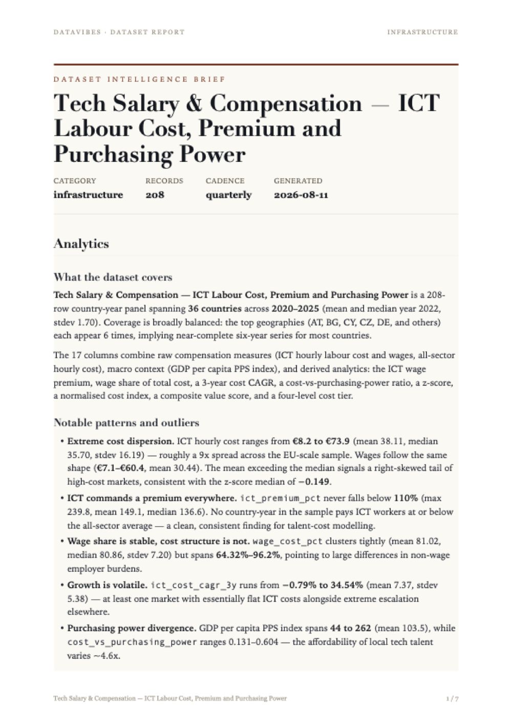
Every issue ships with a written brief: what the data covers, the patterns worth acting on, and the statistical work behind each derived column — with the limitations stated plainly rather than buried.
The page shown here is the first of the full report included in your download. Tap it to read at full size.
Method and limitations
Overview
The tech-salary-compensation dataset (208 rows, 36 countries × up to 6 years, 2020–2025) assembles ICT-sector labour cost indicators alongside economy-wide labour cost and purchasing-power context. Each row is a country-year observation keyed on geo_code + year. The statistical work consists of a preparation stage (normalisation, joining, filtering, sorting) followed by six derived measures, one composite score, one categorical classification and one boolean flag.
Data Preparation
- Normalize — harmonisation of incoming fields prior to combination.
- Join on the composite key
['geo_code', 'year']— merges the ICT-specific labour cost series with all-sector labour cost and the GDP per capita PPS index onto a single country-year grain. - Filter — retains only rows where
ict_hourly_cost_euris non-null. This makes ICT hourly cost the anchor variable: all 208 surviving rows have it populated, while joined-in columns retain gaps (all_sector_hourly_cost_eur203/208;gdp_per_capita_pps_index207/208). - Sort by
geo_code, thenyear— establishes the chronological ordering within each country required for the subsequent panel (growth-rate) derivation.
Derived Metrics
ICT premium (ict_premium_pct, %)
A share of ICT hourly labour cost against all-sector hourly labour cost for the same country-year:
ict_premium_pct = share(ict_hourly_cost_eur, all_sector_hourly_cost_eur)
Expressed as a percentage where 100 would mean parity. The observed floor of 110% and mean of 149.1% indicate ICT labour cost exceeds the whole-economy average in every observation present, ranging up to 239.8%. Coverage is 203/208, inheriting the missingness of the denominator.
Wage share of labour cost (wage_cost_pct, %)
wage_cost_pct = share(ict_hourly_wages_eur, ict_hourly_cost_eur)
The proportion of total ICT hourly labour cost accounted for by wages and salaries, with the residual representing non-wage components (employer social contributions and similar). Fully populated (208/208), mean 81.02%, range 64.32–96.20%, standard deviation 7.20 — a comparatively tight distribution.
Three-year compound annual growth rate (ict_cost_cagr_3y, %)
ict_cost_cagr_3y = cagr(ict_hourly_cost_eur, years=3) computed by geo_code, i.e. as a within-country panel operation over the sorted year sequence.
This is the only metric requiring a time window, and consequently the sparsest: 102/208 non-null (49%), because early years in each country's series lack the three-year lookback. Mean 7.37%, median 6.85%, range −0.79% to 34.54%.
Cost relative to purchasing power (cost_vs_purchasing_power)
cost_vs_purchasing_power = ratio(ict_hourly_cost_eur, gdp_per_capita_pps_index)
A simple ratio of nominal EUR hourly cost to the PPS-based GDP per capita index, intended as an affordability/relative-expense signal. Coverage 207/208. Values are near-symmetric (mean 0.3674, median 0.3699, sd 0.0956), spanning 0.131–0.604.
Standardisation and normalisation of cost
Two rescalings of the same anchor variable were produced:
cost_zscore = zscore(ict_hourly_cost_eur)— mean ≈ 0 (1.79e-16, confirming correct centring), sd = 1, range −1.848 to 2.211. The negative median (−0.149) reflects right skew in the underlying cost distribution.cost_index = minmax_normalize(ict_hourly_cost_eur)— bounded [0, 1] by construction, mean 0.4553, median 0.4186. The same right skew carries through.
Both are computed over the pooled set of country-year rows, not within year or within country.
Composite Scoring
value_score is a weighted linear combination scaled to 100:
| Input | Weight |
|---|---|
cost_index | 0.6 |
gdp_per_capita_pps_index | 0.4 |
Resulting distribution: min 2.75, max 93.59, mean 38.29, median 33.79, sd 21.16. The score is right-skewed (mean above median) and has the widest dispersion of any derived field.
Classification and Flagging
Cost tier — ict_hourly_cost_eur is binned with ordered lower-bound thresholds (EUR/hour), default unknown:
| Tier | Rule | Count |
|---|---|---|
| premium | ≥ 45 | 81 |
| high | ≥ 30 | 41 |
| mid | ≥ 15 | 80 |
| low-cost | below 15 | 6 |
Four distinct labels appear; no rows fell to unknown, consistent with the filter guaranteeing a non-null cost value.
Above-median flag — is_above_eu_median_cost = (cost_index > 0.5), yielding 92 True / 116 False. Note this is a threshold on the min-max index at its midpoint, not on the empirical median.
A final validate step closes the pipeline.
Limitations
- Uneven coverage across derived fields.
ict_cost_cagr_3yexists for only 102 of 208 rows (49%). Any cross-country comparison of growth is effectively restricted to later years and to countries with continuous history; aggregate statistics on this column describe a biased subsample, not the full panel. - Missingness propagates from denominators.
ict_premium_pct(203) andcost_vs_purchasing_power/gdp_per_capita_pps_index(207) are gapped wherever the joined all-sector cost or PPS index is absent. The filter protected only the numerator. - The flag name overstates what is computed.
is_above_eu_median_costtestscost_index > 0.5, the midpoint of the min-max range, which is not the median. Given the right-skewed cost distribution (cost_indexmedian 0.4186,cost_zscoremedian −0.149), the midpoint sits above the median, so the flag under-counts genuinely above-median observations. The 92/116 split should not be read as a median split. - Composite score mixes unlike scales.
value_scorecombinescost_index(bounded 0–1) withgdp_per_capita_pps_index(unbounded index, range 44–262, sd 41.7) without documented rescaling of the second input. The 0.6/0.4 nominal weights therefore do not correspond to 0.6/0.4 influence on the outcome; the higher-variance PPS index will dominate. The weights themselves are stated, not empirically derived. - Score direction is ambiguous. A "value" score that increases with cost (
cost_index, weight 0.6) is not self-explanatory — no inversion step is recorded, so highervalue_scoremeans higher cost as well as higher GDP per capita. Interpretation requires external definition. - Pooled standardisation across years.
cost_zscoreandcost_indexare computed over all country-years together. In a period of nominal EUR cost growth (median 3-year CAGR 6.85%), later years are mechanically pushed toward higher indices independent of any change in a country's relative position.cost_tierthresholds are likewise fixed in nominal EUR, so tier membership can shift through inflation alone; tier counts are not comparable across years. - Fixed nominal bins produce an uneven distribution. The tier cut-points concentrate 161 of 208 rows in
premiumandmidwhilelow-costholds only 6, limiting the discriminatory value of the classification at the bottom of the range. - Ratio metrics lack unit coherence.
cost_vs_purchasing_powerdivides EUR/hour by a unitless index; it is usable for ranking but the absolute values carry no direct interpretation. - Unspecified upstream operations. The
normalizeandvalidatesteps are recorded without parameters, so the specific harmonisation rules and the validation criteria (and what, if anything, failed them) cannot be assessed from the profile. - Panel is short and unbalanced. Six years (2020–2025) across 36 countries gives at most 216 cells against 208 observed rows; the top-frequency countries show 6 rows each, but the shortfall implies some countries are incomplete. No causal or trend inference should be drawn from a window this short, particularly one spanning 2020.
Provenance
Source: Eurostat: lc_lci_lev (labour cost levels by NACE), tec00114 (GDP per capita in PPS)
Licence: Eurostat open data — free reuse with attribution (CC-BY-4.0 equivalent)
Collected and derived with datavibes, a deterministic pipeline: the same config and timestamp always reproduce the same file.